Basics

This page introduces the general framework of the EnerGNN library.

• It introduces Amortized Optimization [1], which encompasses traditional supervised learning.

• It explains how to implement your own use case using the energnn.problem interface.

• It outlines the core features of our energnn.graph data representation module.

• It gives some details about the GNN architectures implemented in energnn.model.

• It shows how to train a GNN model over your own use case using the energnn.train module.

[1] Brandon Amos, Tutorial on Amortized Optimization, 2022.

---

Amortized Optimization

Consider an optimization problem formulated as follows:

\[\begin{align} y^\star(x) \in \arg \min _y \ f(y;x), \end{align}\]

where:

• \(x\) is a context graph (input data),

• \(y\) is a decision graph (output data),

• \(f\) is the objective function to minimize.

We seek to solve this problem for a distribution of contexts \(x \sim p\), using a trainable GNN model \(\hat{y}_\theta\), parameterized by \(\theta\). This leads to the following Amortized Optimization [1] problem:

\[\begin{align} \theta^\star \in \arg \min _\theta \ \mathbb{E}_{x \sim p} [f(\hat{y}_\theta(x);x)]. \end{align}\]

EnerGNN addresses this learning problem via the following general training loop:

\[\begin{split}\begin{align} x &\sim p & & \text{(1) Context sampling}\\ \hat{y} &\gets \hat{y}_\theta(x) & & \text{(2) Decision inference} \\ \hat{g} &\gets \nabla_y f(\hat{y};x) & & \text{(3) Gradient estimation} \\ \theta &\gets \theta - \alpha J_\theta[\hat{y}_\theta]^\top.\hat{g} & & \text{(4) Back-propagation} \end{align}\end{split}\]

EnerGNN handles steps (2) and (4), which are independent of the use case, while steps (1) and (3) are use case specific and should respect the provided energnn.problem interface.

---

Implementing your own Use Case

Attention

Should you use EnerGNN?

EnerGNN has been designed for Amortized Optimization problems where the objective function \(f\) is permutation-invariant (i.e., for any permutation \(\sigma\), \(f(\sigma(y); \sigma(x)) = f(y; x)\)). This entails that the solution \(y^\star\) is permutation-equivariant (i.e., for any permutation \(\sigma\), \(y^\star(\sigma(x)) = \sigma(y^\star(x))\)). If this property is not satisfied, then resorting to a GNN is probably not a good idea.

The energnn.problem API provides an interface to integrate your own use cases. A general overview is provided below, and an in-depth guide is available in Use Case Implementation.

Problem

The Problem class defines a single instance of the optimization problem. It must implement:

• context_structure: General structure of contexts \(x\).

• decision_structure: General structure that decisions \(y\) should respect. Notice that gradients \(\nabla_y f\) share the same structure.

• get_context(): Returns the context graph \(x\).

• get_gradient(): Computes the gradient \(\nabla_y f\) for a given decision \(y\). Depending on the use-case, the gradient can either be straightforward to compute, or require more expensive Monte-Carlo computations.

• get_score(): Evaluates the quality of a decision (which may or may not coincide with the objective function).

ProblemBatch

For training, problems are grouped into a ProblemBatch. The interface is the same as for Problem, but contexts, decisions and gradients are batched together.

ProblemLoader

The ProblemLoader is the iterator that provides these batches to the training engine.

for problem_batch in train_loader:
    context, _ = problem_batch.get_context()
    # Do stuff.
    ...

---

Data Representation using H2MG

Contexts \(x\), decisions \(y\), and gradients \(\nabla_y f\) are all represented as H2MGs (Hyper Heterogeneous Multi Graphs).

• Hyper graphs. Made of hyper-edges that can connect more than 2 entities.

• Heterogeneous graphs. Multiple component types (e.g., lines, transformers, etc.).

• Multi graphs. Multiple components can be collocated.

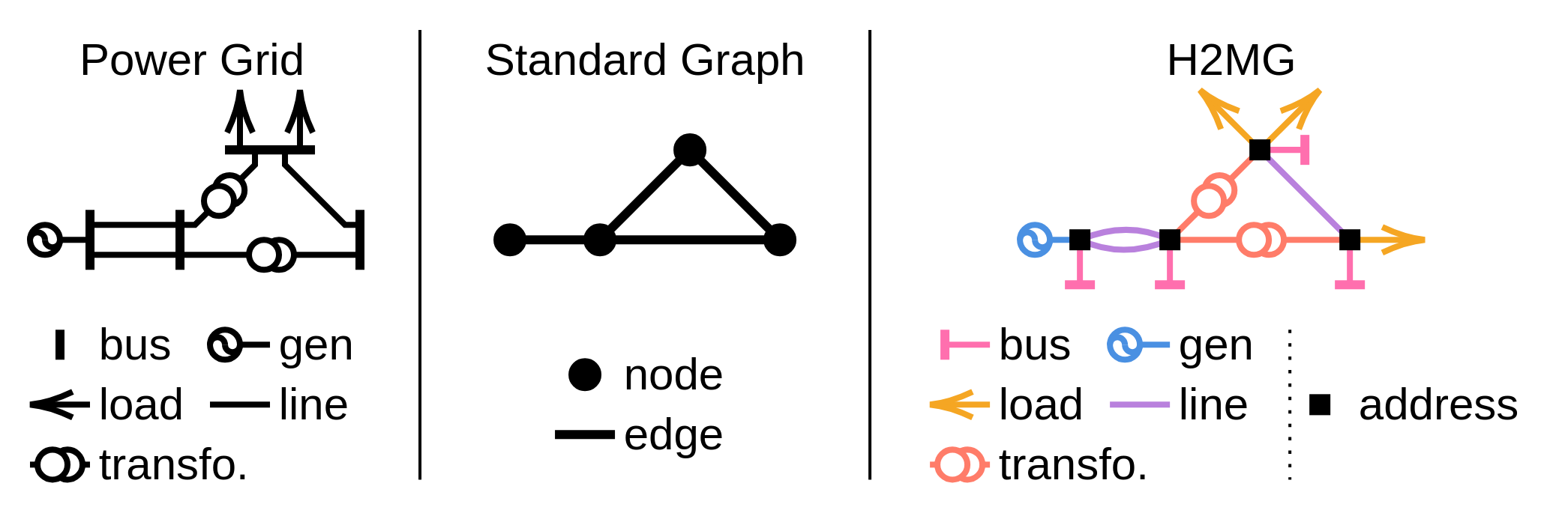
H2MGs are made of hyper-edges (i.e. objects), which are interconnected via addresses. These addresses do not bear any numerical feature, and only serve as interface between hyper-edges, as illustrated by the figure above. All hyper-edges of the same class share the same feature and port keys. The order of an hyper-edge is the cardinality of its ports.

In practice, a Graph is a dictionary of HyperEdgeSet objects. For computations with JAX, we use energnn.graph.JaxGraph, which is an optimized version compatible with automatic differentiation.

See the Tutorial for an example of H2MG data.

---

Graph Neural Network Models

EnerGNN provides a modular and parametrizable GNN library designed to natively process H2MG data. The main model, GNN, follows a modular pipeline:

1. Normalizer. Adjusts the distribution of input features (e.g., uniformly distributed between -1 and 1).

2. Encoder. Embeds input features into a latent space.

3. Coupler. Handles information propagation (e.g., via iterative message passing) over the graph structure.

4. Decoder. Produces the final decision from coupled latent representations.

All modules inherit from flax.nnx.Module, allowing great flexibility and perfect integration with the JAX ecosystem.

Ready-to-use GNN implementations are available in energnn.model.ready_to_use.

from energnn.model.ready_to_use import TinyRecurrentEquivariantGNN

model = TinyRecurrentEquivariantGNN(
    in_structure=problem.context_structure,
    out_structure=problem.decision_structure
)
context, _ = problem.get_context()
decision, _ = model(context)

Notice that the GNN needs to know about the context and decision structures defined by the use-case.

---

Trainer

The Trainer orchestrates the learning process. It takes as input a model, a gradient transformation (via optax), and handles the training loop.

import optax

trainer = Trainer(model=model, gradient_transformation=optax.adam(1e-3))
trainer.train(train_loader=loader, n_epochs=10)

Additionally, evaluation can be periodically run, checkpoints can be saved using orbax, and score / infos can be monitored using an experiment tracker.

import orbax.checkpoint as ocp

checkpoint_manager = ocp.CheckpointManager(directory="tmp")
my_tracker = ...  # Implement your own

trainer.train(
    train_loader=train_loader,
    val_loader=val_loader,
    checkpoint_manager=checkpoint_manager,
    tracker=my_tracker,
    n_epochs=10
)

---

Next Steps

Now that you are familiar with the basics, you can:

• Follow the Tutorial for a hands-on example.

• Learn how to implement a Use Case Implementation.

• Explore the API reference for detailed API information.